
You already run a randomized logging policy. Each matured decision carries the action taken, the probability that policy assigned to it, the options that were legal that day, and the person context known at choice time. A natural next question is: what would a candidate per-person policy have earned on that same traffic?
That question is offline policy evaluation. It is not a live A/B test against holdout, and it is not a promise that tomorrow’s traffic will match yesterday’s log. Done carefully, it can still be a useful guarded preview: an estimate of how the candidate would have scored, plus overlap checks and a sequential range a buyer can use to set a decision rule.
BanditBuzz’s preview uses five person-level folds and a doubly robust estimator. The product stays in collecting until it has enough context-bearing rows, enough effective sample size, and no extreme importance weight. Those checks alone control the current ready label. The preview also reports a 95% confidence sequence, but the checkout path does not yet require its lower bound to be positive. The rest of this post explains the estimator, the fold flow, that product gap, and the limits that keep the claim from sounding stronger than the method.
What the preview is estimating
Name the estimand before reading a number.
The free standard policy, call it μ, is the logging policy. It chooses among offered options with Beta-Bernoulli Thompson sampling and writes the chosen action’s probability into the decision log. Holdout rows are excluded from this preview. Replay uses matured, non-holdout decisions that the standard policy made with decision-time context available and a positive logged probability.
The candidate is a hierarchical linear Thompson policy, call it π. It uses a small fixed feature vector (intercept, credit proxy, outcome probability, persona indicators, and missing-value flags) and a Gaussian linear reward model. That model is a compact first approximation, not a claim that reward is truly linear or Gaussian. Predicted means used in replay are clamped to the unit interval.
The preview asks for the change in matured reward rate if π had chosen on those same logged rows, compared with the reward rate actually observed under μ. It reports:
- the observed standard reward rate on the context rows
- the estimated contextual reward rate under π
- their absolute difference
- relative lift when the baseline is nonzero
- a 95% asymptotic confidence sequence for the absolute difference
- context coverage, effective sample size, and the largest importance weight
It is a replay against the free logging policy, not against holdout. Holdout answers a different question: whether the live whole policy beats its control choice. Mixing those two estimands is how a preview gets sold as a finished experiment.
Why a reward model alone is not enough
If every logged row came with a perfect model of expected reward for every action under every context, you could score π by averaging the model’s prediction under π’s action probabilities. Real reward models are wrong. A biased direct method will invent lift.
The other extreme is inverse propensity scoring alone: reweight each observed reward by how often π would have chosen the logged action relative to how often μ did. That needs accurate logging probabilities and enough overlap. When π puts mass where μ almost never acted, weights explode and variance eats the estimate.
Dudík, Langford, and Li (2011) study exactly this setting: evaluating a new policy from historic contexts, actions, and partially observed rewards. Their abstract states the trap plainly: previous approaches “rely either on models of rewards or models of the past policy. The former are plagued by a large bias whereas the latter have a large variance.” Their doubly robust estimator combines both pieces so that the estimate stays accurate when either the reward model or the past-policy model is good.
Li, Chu, Langford, and Schapire (2010) made the operational point earlier in a news-recommendation study: payoffs are observed only for the arms the logging policy chose, so evaluating a different policy from that log is not a simple average of observed clicks. Randomized logging and stored probabilities are what make the later estimator possible.
Public logged-bandit benchmarks keep the same discipline. The Open Bandit Dataset and Pipeline release real fashion-recommendation traffic with known behavior policies so researchers can compare offline estimators against on-policy ground truth. That program only works when the log carries the randomization record. BanditBuzz’s production path has synthetic and production tests for replay, but it does not yet ship a public benchmark suite of its own. Saito et al. are the external reference for what that suite should look like.
The estimator in plain language
For one logged decision with context x, taken action a, reward r, and logging probability μ(a | x), the held-out fold supplies:
- π(· | x): Monte Carlo action probabilities under the candidate policy for that row’s offered set
- q(x, a): the fold’s direct prediction of expected reward for the logged action, clamped to 0-1
- q(x, π): the expected direct prediction under π, that is Σ_a′ π(a′ | x) q(x, a′)
The doubly robust score for that row is:
q(x, π) + [π(a | x) / μ(a | x)] × (r − q(x, a))
Read it as two parts:
- Direct piece. Start from what the reward model says π would earn on this person: q(x, π).
- Correction piece. Look at the action that actually happened. Compare the observed reward r to what the model expected for that logged action, q(x, a). Scale that residual by the importance weight w = π(a | x) / μ(a | x), which says how much more (or less) often the candidate would have chosen that same action.
If the reward model is perfect, the residual is noise around zero and the correction averages out. If the propensity model is perfect and overlap is decent, the weighted residual corrects a bad q. You still need both pieces to be serviceable in production, which is why BanditBuzz refuses to report a finished preview when weights are wild.
Logged row under μ
        │
        ▼
   Build q and π on other folds
        │
        ├─► direct:   expected reward if π had chosen
        └─► correct:  weight × (observed reward − q on logged action)
                │
                ▼
        one doubly robust score per row
The preview’s contextual reward rate is the mean of those scores. The baseline is the mean of the observed rewards on the same rows. The difference series (score minus observed reward on each row) feeds the confidence sequence.
Five person-level folds
Cross-fitting limits what the reward model can learn from the row it scores.
People are assigned to five stable folds with a deterministic hash of the stable person key (or the decision id when no key exists). For each fold index k:
- Fit the hierarchical linear model on matured training rows whose fold is not k.
- Wrap that model in a candidate Linear Thompson policy whose Monte Carlo draws use a fold-specific seed.
- Score only the held-out replay rows in fold k: non-holdout standard-policy decisions with context, an offered set, and a positive logging probability.
- For each held-out row, compute π, q, the importance weight, and the doubly robust score from that fold’s policy alone.
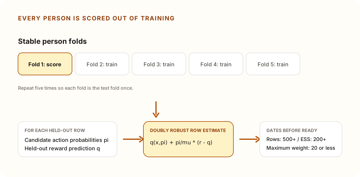
Five-fold cross-fitting. No person trains the fold-specific policy that scores their rows.
Folds are person-level, not time-blocked. A person who appears many times stays inside one fold, so their rows do not train the model that scores them. That reduces a simple form of overfitting. It does not create a calendar holdout, and it does not remove within-person dependence from the uncertainty calculation.
Training and scoring use the context snapshot stored on the decision, never a later lookup. That prevents the preview from adding features learned after the reward arrived. Upstream score construction still needs its own time-leakage checks.
Action replay leaves the logged timing process in place. Timing has a separate preview that conditions on an accepted action. There is no joint action-by-time replay that multiplies both propensities today.
Overlap gates before any “ready” label
Importance weights are w = π / μ. BanditBuzz does not clip them. Clipping would hide the worst mismatches between candidate and logging policy. Instead the product stays in collecting unless all of these hold:
| Gate | Threshold | Why it exists |
|---|---|---|
| Context-bearing decisions | at least 500 | Sparse context makes both q and π fragile. |
| Effective sample size | at least 200 | For weights w, ESS = (Σw)² / Σw². Low ESS means a few rows dominate. |
| Maximum importance weight | at most 20 | A single extreme weight is a hard stop, even if ESS looks fine. |
The product reports ESS and the largest weight. It does not yet show the full weight distribution. Coverage (share of eligible decisions that had context) is reported for diagnosis; it is not itself an offer gate.
Until those gates clear, baseline and contextual rates, the difference, the confidence bounds, and lift stay null. The scoreboard can show that collection continues. It should not show a half-finished lift as a purchase signal.
A sound buying rule uses the confidence sequence
When the gates pass, BanditBuzz builds a 95% asymptotic confidence sequence for the mean of (doubly robust score − observed reward) across the context rows. The production boundary follows Maharaj et al. (2023), equation 1, with their production tuning value ρ² = 0.001. That paper describes anytime-valid sequences used on an enterprise A/B platform: a range meant for repeated inspection, not a single fixed-sample test at a pre-registered end date.
For a cautious buying rule, require the lower bound of that sequence for the absolute reward-rate change to be strictly above zero. A positive point estimate is not enough. A lower bound that touches zero is not enough.
The current product does not enforce that rule at checkout. status: "ready" means only that the 500-row, ESS, and maximum-weight checks passed. A buyer can subscribe with a negative or unresolved lower bound. That is a real gap between the research rule and the money path, and it should stay visible until the API enforces it.
Even with that rule, coverage may not survive every production complication. The landing research and data-science brief are frank: coverage under repeated people, estimated propensities, and nightly refits still needs a public simulation benchmark. The sequence is the best current product choice for a dashboard people open more than once, not a finished proof of sequential validity for this exact replay pipeline.
Limits that belong next to the estimate
Replay is a preview. Treat these limits as part of the method, not footnotes.
Not a live result. The estimate answers how π would have scored on logged μ traffic. It does not measure π on live traffic, and it does not replace the stable person-level holdout that measures the live whole policy against control.
Unit is a decision. One person can contribute many matured decisions. The current range does not cluster by person. Dependence within a person can make intervals look tighter than a person-level analysis would.
Propensities are estimates. Holdout probabilities are exact. Thompson probabilities use 500 Monte Carlo draws from the same scoring rule used to choose, then one-count smoothing. They are not exact integrals and they are not clipped. Dudík et al. require a useful model of the past policy; Monte Carlo noise in μ is one more reason the weight caps exist.
Nightly refits. Attribution, maturation, contextual fitting, and replay run in batch. Long reward windows plus batch lag slow learning. The fold policies used for preview are rebuilt on that cadence. There is no claim of a finite-time regret bound for this delayed loop.
Model misspecification. The contextual reward model is linear-Gaussian, including for binary rewards. Displayed expected rewards used in q are clamped to 0-1. Logistic Thompson sampling remains a research target (Gouverneur et al., 2024), not the live policy. Fixed ridge strengths are product settings, not learned hyperparameters.
Option sets are row-local. Replay scores π only over the options offered on that row. Adding or removing an option does not rewrite old rows. Changing the reward definition creates a new decision-point version and a new learning problem.
No buyer export yet. Each choice records version, offered set, selected option, propensities, context snapshot, and maturation state. There is not yet a full evaluation-log export or a supported external replay package. Historical posterior snapshots that would reproduce every past random draw are also not provided.
Drift. Action posteriors and the contextual action model currently use full history. Timing alone uses a 90-day window. Sliding-window and discounted policies (Fiandri, Metelli, and Trovò, 2024) are next tests, not the current action-replay method.
How to read a ready preview
When status flips to ready, read in this order:
- Context coverage and row count. Confirm you are looking at enough context-bearing decisions, not a thin slice of identified traffic.
- ESS and max weight. If either is near its gate, treat the estimate as fragile even though it cleared the bar.
- Baseline and contextual rates. These are rates on the same logged rows under μ’s outcomes and π’s doubly robust scores.
- Absolute difference and its sequence. Use the lower bound of the absolute change as your own buying rule.
- Relative lift last. Lift is useful packaging when the baseline is stable. It does not control the current checkout path.
Then ask the human questions the math does not answer. Did the offered set stay roughly comparable over the collection window? Did reward definitions stay inside one version? Are you about to treat a replay against μ as if it were a holdout win?
What this method is for
Person-level cross-fitting plus a doubly robust estimate can form a guarded preview of a contextual policy before it spends live traffic. The honesty comes from the parts people skip in a demo: stored logging probabilities, decision-time context snapshots, unclipped weights with hard caps, a minimum effective sample size, and a sequential range. Today the buyer, not checkout code, must require a positive lower bound.
The method does not abolish model error, propensity estimation error, repeated-person dependence, or nightly batch lag. It names them, refuses to ship a number when overlap fails, and keeps the estimand distinct from live holdout lift. That is the useful standard for a data scientist who already trusts experiments and is newly responsible for off-policy evaluation: derive intuition, keep the gates visible, and do not confuse a replay with a live result.